AN INTERACTIVE RESEARCH ESSAY EMAD MOSTAQUE · 2026
FROM CHIRALITY TO THE STANDARD MODEL
What if handedness fixed the structure of matter?
The electron in an atom belongs to a pattern that repeats across three families of matter. The weak interaction treats left and right differently. This is a journey from those discoveries to a mathematical question: could a common origin fix the pattern?
Choose what to open first. The page rearranges around the questions you bring.
10 CHAPTERS · EQUATIONS FOLDED AWAY
Begin with a world that distinguishes left from right.
Start with Wu’s experiment. Learn what symmetries and representations mean, see how they describe the particles we measure, then follow the paper’s search for a common origin. The equations open when you want them.
CHOOSE YOUR DEPTH
The same argument, with more detail when you want it.
A QUESTION WITH A HISTORY
Nature distinguishes left from right.
Put your hands together. They match as mirror images, but you cannot turn one into the other. Physicists once expected the laws of nature to treat a process and its mirror image alike. Wu’s experiment showed that the weak interaction does not.
CHIEN-SHIUNG WU1912—1997
AI-generated historical interpretation, based on a portrait from the AIP Emilio Segrè Visual Archives, Segrè Collection. Source · CC BY 4.0; stylised and recomposed. The apparatus is illustrative.
1956
Ask whether the mirror rule was ever tested
Tsung-Dao Lee and Chen-Ning Yang examined the evidence for parity conservation. For the weak interaction, the decisive experiments were missing. They proposed ways to test what had been treated as a general rule of nature.
Wu and her National Bureau of Standards collaborators found that electrons from polarised cobalt-60 nuclei preferred one direction relative to the nuclear spin. Their experiment established parity violation in beta decay: the weak interaction distinguishes a process from its mirror image.
Wu’s team aligned the nuclear spins and measured where the electrons went. More emerged opposite the spin. A spatial inversion reverses the electron directions but leaves spin, an axial vector, unchanged. The two patterns differ.
Illustrative angular pattern, not measured data. The shape exaggerates the asymmetry to make it visible.
BEFORE THE PARTICLES: A LANGUAGE FOR SYMMETRY
A small turn can tell you about the whole.
Turn a perfect sphere and it still looks the same. You can turn it a little, then a little more. Those continuous transformations form a , named after the Norwegian mathematician Sophus Lie.
In the 1870s, Lie developed a way to study such transformations through their infinitesimal changes. A records those tiny motions and how they combine. For rotations, the order matters: turn a book about one axis and then another, and reversing the order generally gives a different result.
Killing and Cartan’s classification is exhaustive. Every finite-dimensional compact simple Lie algebra belongs to one of four infinite series, Aₙ, Bₙ, Cₙ and Dₙ, or five exceptional types: G₂, F₄, E₆, E₇ and E₈. There is no further compact simple type outside this list. Allowing direct sums and commuting central directions extends the catalogue to every finite-dimensional compact Lie algebra. A sum of simple factors is called semisimple; the abelian centre is the additional part that commutes with the whole algebra.
That completeness matters here. The paper starts with the full compact domain, then studies embeddings and their representations under its two conditions. The catalogue supplies every possible building block; the paper’s reduction and anomaly test determine what survives. Classification and compact forms, MIT notes §§22–23, 39, 42 ↗
A representation tells us how a symmetry acts on a set of fields. The Standard Model’s charges are representation data. In this paper, the remaining directions of a larger algebra supply the representation, so the symmetry and its proposed matter content are tied together from the start.
Continuous symmetry, illustrated. These are internal mathematical directions in the paper, not extra dimensions of space.
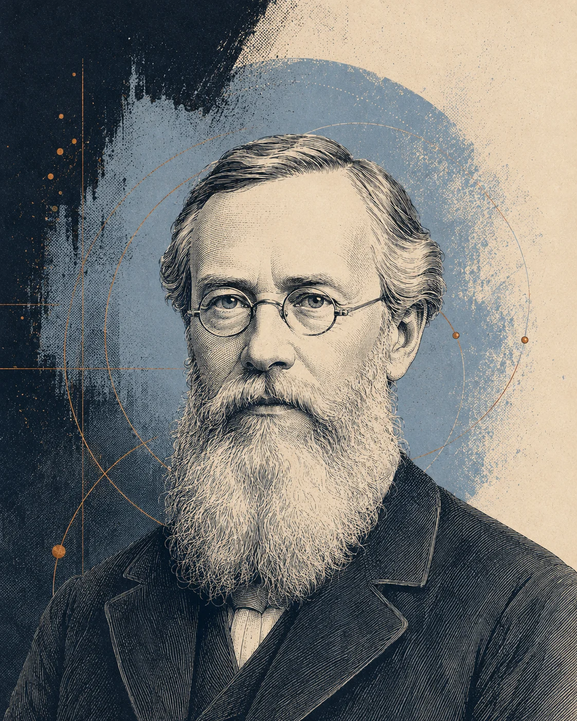
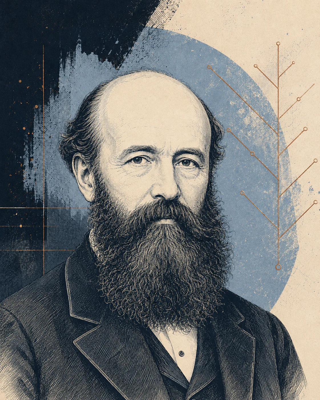
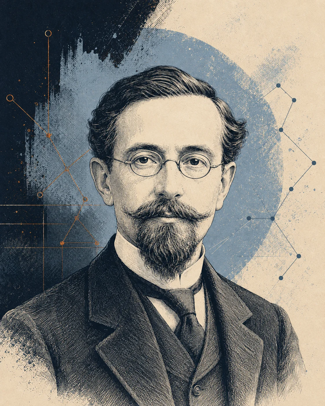
Illustrated historical portraits. Dates identify the work described, not the age shown in each portrait.
FROM THE EXPERIMENT TO ITS DESCRIPTION
Left and right follow different weak-interaction rules.
In the Standard Model, left- and right-chiral fermion fields transform differently under the weak gauge symmetry. “Chiral” describes this handed structure. Lie algebras and their representations let us write down exactly how it works.
The experiment establishes an asymmetry in nature. To describe it precisely, we need to know how a symmetry acts on a field. Begin with a transformation you can move yourself.
A LANGUAGE FOR MATTER
From a small turn to a particle’s charges.
Rotate an experiment and its orientation changes. If the physical laws stay the same, that transformation is a symmetry. Lie theory gives us a language for continuous symmetries. Representation theory tells us how they act on the things we want to describe.
Particle physics uses this language for internal transformations too. These mix components of fields, rather than turning an object in space. The familiar rotation below gives us a way to learn the rules before applying them to particle charges.
01 / A GROUP AND ITS ALGEBRA
Two turns. Does the order matter?
Start with the same gold arrow. Turn it about the x-axis, then the z-axis. Now reverse the order. At most angles, the arrow ends somewhere else.
All rotations of three-dimensional space about the origin form the Lie group SO(3). You can combine rotations, undo them, and vary the angle continuously. Its Lie algebra describes the infinitesimal turns: the basic directions of change from which finite rotations can be built.
Each basic direction is a generator. The Lie bracket records how two such changes fail to commute. Here, doing the turns in a different order gives a different result. That rule is part of the algebra’s structure.
X, THEN Z
Z, THEN X
Endpoint separation: 0.502 unit lengths. Try 0°, then 90°.
From the picture to the bracket +
For matrix generators X and Z, the Lie bracket is [Z,X] = ZX − XZ. Expanding the two orders gives etZetX − etXetZ = t²[Z,X] + O(t³). The first-order turns agree; their second-order difference remembers the order.
The displayed rotations act on ordinary three-dimensional vectors. The paper uses internal symmetries acting on field components. The mathematical language is shared; internal dimensions are not additional spatial directions.
02 / HOW A SYMMETRY ACTS
One transformation. Different responses.
A symmetry alone does not tell us what matter exists. We also need its representation: the rule telling each field how to respond to that symmetry.
For the circle group U(1), charge fixes how fast a field’s complex phase turns. A charge-two field turns twice as far as a charge-one field under the same transformation. The arrows below are complex amplitudes, not spinning particles.
CHARGE 1
CHARGE 2
Representation, irreducibility and complex type +
A smooth finite-dimensional group representation is a map ρ: G → GL(V) with ρ(g₁g₂) = ρ(g₁)ρ(g₂). Differentiating it gives a Lie-algebra representation, preserving brackets. Its dimension counts components in V, not copies of a family or dimensions of spacetime.
An irreducible representation has no proper nonzero invariant subspace under the full group. A weak doublet is irreducible under SU(2), although a single chosen rotation can be diagonalised. The two U(1) examples above are separate one-dimensional representations.
“Complex type” is stronger than having complex entries: the representation is inequivalent to its conjugate. The SU(2) doublet is pseudoreal, not complex type. The paper instead starts with a real irreducible adjoint complement q whose commuting endomorphisms form ℂ. Its complexification is V ⊕ V*, with V and V* inequivalent.
KEEP THREE IDEAS SEPARATE
The symmetry. Its action. The number of copies.
An algebra supplies the transformation rules. A representation realises those rules as matrices acting on components. We can then have several fields with the same transformation rules. These are three different choices, and three different counts.
Generators and representation dimensions count different things.
Symmetry
Generators
A representation
Components
SU(2)
3
Weak doublet
2
SU(3)
8
Colour triplet
3
E₆
78
The 27 used in the paper
27
SU(2), for example, has three independent generators. On a doublet, each is represented by a 2 × 2 matrix. Three families of doublets would be three copies of that two-component representation.
What are the adjoint and the Killing–Cartan list? +
An algebra can act on itself: a generator X changes another element Z through the bracket [X,Z]. This is the adjoint representation, whose dimension equals the number of generators. The eight gluons carry the adjoint colour index; quarks carry a three-component colour index instead.
The Killing–Cartan classification is complete for finite-dimensional complex simple Lie algebras, equivalently for compact real simple Lie algebras: Aₙ, Bₙ, Cₙ, Dₙ and G₂, F₄, E₆, E₇, E₈. “Simple” means non-abelian with no nonzero proper ideal, an algebraic part preserved by brackets with everything else.
A semisimple Lie algebra is a finite direct sum of simple Lie algebras. The factors commute with one another. A simple algebra is the one-factor case; e₆ ⊕ su(3) is an example with two factors. Every finite-dimensional compact Lie algebra splits into a semisimple part and an abelian centre. The centre commutes with the entire algebra. This includes arbitrary finite ranks, sums and repetitions. The classification exhausts the algebras; specifying embeddings, representations and global group identifications is further mathematical work.
The paper links these choices by putting a smaller algebra inside a larger one and letting the smaller algebra act on all the remaining directions. This remaining space is its adjoint complement. The classification asks when that space has the specified chiral and cubic-anomaly properties.
We have the language: an algebra gives transformation rules, a representation tells us how a field follows them. Now meet the Standard Model and work out the charges of an electron and its quark neighbours.
THE PHYSICS BEHIND THE QUESTION
The Standard Model. A pattern in the world.
The matter in an atom, the light it emits, and the weak processes that change one kind of particle into another are described by a remarkably small set of fields and interaction rules. Those rules carry a mathematical pattern we can learn to read.
START WITH AN ATOM
A few fields. An extraordinary amount of the world.
Electrons surround an atom’s nucleus. Inside it, protons and neutrons contain up and down quarks, bound by the strong interaction. Light is made of photons. The Standard Model brings these ingredients into one quantum field theory, together with their heavier relatives, neutrinos and the fields responsible for the weak interaction and the Higgs mechanism.
A field has a value at every point in spacetime. A particle is a quantum excitation of a field: an electron belongs to the electron field, a photon to the electromagnetic field. To describe their interactions, we need rules for how those fields transform.
Quarks and leptons are fermions. Fermion fields can transform in two chiral ways under spacetime symmetry, called left- and right-handed. The weak interaction treats them differently. The three internal symmetries below describe the charge rules.
SU(3)c
Colour
Each quark has three colour components. Eight gluon fields couple to this charge and to one another, producing the strong interaction. “Colour” names an internal charge, unrelated to visible colour.
SU(2)L
Weak isospin
Left-chiral quarks and leptons come in pairs, such as the electron and its neutrino. The W interaction connects the two components. The right-chiral electron is a singlet instead. This difference is the chiral structure of the weak interaction.
U(1)Y
Hypercharge
Each field also carries a hypercharge, Y. After electroweak symmetry breaking, the hypercharge field and neutral weak field mix to give the photon and Z. Electric charge combines hypercharge with weak isospin: Q = T₃ + Y.
The numbers in SU(3) and SU(2) refer to their defining representations. They count internal components, not families. The observed matter pattern repeats across three generations, a different kind of three. We will keep those counts separate as the argument unfolds.
What makes a symmetry a gauge symmetry? +
U(N) is the group of unitary transformations: matrices that preserve the squared norm of N complex components. SU(N) adds the requirement that the determinant is one. U(1) is a phase rotation, like the turning complex amplitude in the representation exhibit.
We can choose the internal basis used to describe a field separately at each spacetime point. A gauge transformation changes that description while leaving physical observations unchanged. Gauge fields let us compare the descriptions at neighbouring points; requiring this local freedom constrains how the fields interact.
The familiar product SU(3) × SU(2) × U(1) specifies the local symmetry structure. Groups with different global identifications can share the same Lie algebra. The paper checks that its particular embedded Standard Model subgroup has the quotient by ℤ₆. Read about the global forms ↗
The gallery uses L and R for left- and right-chiral fields. Its animated pictures are symbolic; the representation labels give the actual charges. For a refresher on those labels, explore how a representation works ↗
WORK OUT THE CHARGES
Read the label: (1, 2)₋₁/₂
For the left-chiral lepton field, 1 means a colour singlet, 2 means a weak doublet, and −½ is its hypercharge Y. A singlet is unchanged by that group’s transformations; a doublet has two components.
The weak-isospin labels T₃ are +½ and −½; both components share Y. Add the two numbers to find electric charge Q, measured in units of the positive elementary charge. Choose a component below.
The right-chiral electron is (1, 1)−1. It is a weak singlet: T₃ = 0. Its electric charge is also −1, despite its different electroweak representation.
THE PARTICLES WE KNOW
The same charges. Three families.
The electron in an atom has two heavier relatives, the muon and tau. Quarks repeat too. Choose a family, then a particle: the masses change across families, while the gauge-charge pattern repeats.
A closer look at electron
MATTER FIELD
electron
Electric charge −1Spin ½
The left-chiral charged lepton shares a weak doublet with its neutrino. The right-chiral field is a weak singlet. Their electric charges agree; their electroweak representations do not.
Left-chiral field
(1, 2)₋₁/₂
Right-chiral field
(1, 1)₋₁
Charges use SU(3) × SU(2) with hypercharge Y; Q = T₃ + Y. Antiparticles are implicit. W± and the eight gluon fields are grouped in the gallery.
Is chirality the direction a particle spins? +
Chirality labels the two kinds of Weyl spinor under spacetime symmetry. Helicity compares spin with the direction of motion. They agree for massless particles with the usual particle convention; for a massive particle they are different concepts. The L and R glyphs here label field components, not classical rotation.
FROM A RULE TO A MEASUREMENT
How does the mathematics meet reality?
A detector records energy, momentum and particle tracks. The theory predicts the probabilities of different outcomes. Physicists specify the fields and their interactions, measure the parameters, then use the same theory to calculate other processes. Agreement across those tests is what gives the Standard Model its force.
1983
A theory tells an experiment what to look for.
01
The structure
The electroweak theory joins weak isospin and hypercharge. Its Higgs field gives masses to the W and Z while leaving the photon massless.
02
The calculation
With parameters constrained by earlier measurements, the theory predicted massive W and Z bosons and their interactions. Their decays gave experiments identifiable combinations of charged leptons and missing momentum.
03
The observation
UA1 and UA2 found the W and Z at CERN in 1983. The comparison involved masses, event rates and decay patterns, not just the appearance of a new particle.
One equation behind the example +
At leading order: mW = gv/2; mZ = v√(g² + g′²)/2
Here g and g′ are interaction strengths and v is the Higgs vacuum scale. Their values come from measurements; the theory supplies the relationships. Precision comparisons include quantum corrections.
The charge pattern is one of the inputs to this experimentally tested theory. The paper asks why that pattern, and its threefold chiral repetition, might arise from a single algebraic construction. To reach that question, first examine two constraints the pattern already meets: chirality and anomaly cancellation.
WHY THE LEFT/RIGHT DISTINCTION MATTERS
A mass term needs the charges to fit.
An electron’s left- and right-chiral fields carry different electroweak charges. A bare Dirac mass cannot join them while respecting that symmetry. The Higgs field supplies a gauge-invariant interaction; its vacuum value turns that interaction into a mass term.
A closer look at electron
DIFFERENT ELECTROWEAK REPRESENTATIONS
No Higgs background. No Yukawa mass.
Keep the electron’s Yukawa coupling fixed and vary the Higgs background. The bridge shows the strength of the resulting tree-level mass term.
0v = 246 GeV
mₑ = yₑ v / √2mₑ(v) / mₑ(v₀) = 0.00
This varies a background field, not collision energy or temperature. It shows a Lagrangian mass term, not the full behaviour of particles in a hot plasma.
What does the Higgs actually supply? +
The electroweak-invariant interaction is −yₑ L̄ H eR + h.c. The hypercharges add as +½ + ½ − 1 = 0, and the weak-doublet indices contract. With ⟨H⟩ = (0, v/√2), it gives mₑ = yₑv/√2. The same Yukawa interaction exists before symmetry breaking, but its mass contribution vanishes when the background is zero. The value of yₑ remains an input.
This example concerns Dirac masses. A gauge-singlet Weyl fermion can instead admit a Majorana mass. With Standard Model fields, the dimension-five operator schematically written (LH)(LH)/Λ is also gauge-invariant; after symmetry breaking it can generate a Majorana neutrino mass proportional to v²/Λ. The field content and permitted operators decide which possibilities exist. Including this dimension-five operator extends the minimal renormalizable Standard Model. Weinberg, 1979 ↗
A QUANTUM CONSISTENCY TEST
Every piece has to balance.
Quantum loops can spoil a gauge symmetry that works in the classical equations. A consistent gauge theory needs these anomaly contributions to cancel. In one Standard Model family, the quarks and leptons balance each other. Try leaving one out.
For this calculation, every field is written left-handed. The symbols uᶜ, dᶜ and eᶜ are the conjugates of the right-chiral fields above; their gauge charges reverse. Q and L are the quark and lepton doublets.
ONE FAMILY · ALL-LEFT-HANDED CONVENTION
Y³ SUM0CANCELS
SU(3)³0SU(3)²Y0SU(2)²Y0Y³0gravity²Y0
The displayed local anomalies cancel. The number of weak doublets is even, so the usual SU(2) global-anomaly test also passes.
4 weak doublets
The bars use integer-rescaled coefficients, with q = 6Y. A failed sum represents an inconsistency in the proposed theory, not an explosion or collapse of physical matter. Repeating a complete family preserves cancellation, so this test alone does not select three generations.
Follow the exact arithmetic +
For Y³, sum dcolour × dweak × q³. A full family gives 6 − 192 + 24 − 54 + 216 = 0. For the mixed gravitational anomaly, use q rather than q³. For SU(3)²Y and SU(2)²Y, the displayed coefficients absorb the common fundamental Dynkin index. The SU(3)³ channel assigns opposite signs to a fundamental and its conjugate. The SU(2) global check counts colour copies of weak doublets. uᶜ, dᶜ and eᶜ denote left-handed conjugates of the right-chiral particle fields shown above.
NOW REVERSE THE USUAL QUESTION
What if the matter and its symmetry came from the same structure?
In the Standard Model, we specify the symmetry, assign the matter representations and repeat the family pattern three times. The paper ties those choices together: place one compact algebra inside another, and use all the remaining directions as a representation of the smaller one. This adjoint complement must be irreducible and of . Requiring a nonzero cubic-anomaly radical as well leaves one pair. We can now follow the conditions that make that uniqueness possible.
The particle pattern and its consistency tests were built from experiment and theory. How much does an ordinary unification scheme determine, and which choices does it leave open?
HOW THE PATTERN WAS BUILT
Knowing the pattern. Asking why this one.
The Standard Model was built through a conversation between experiment and theory. It describes a remarkable amount with a small set of symmetry rules. Explaining why those rules and those matter representations occur is a further question.
Glashow · Weinberg · Salam. Illustrated later-life portraits, not a scene from the 1960s.
THE ELECTROWEAK THREAD
A theory links light and weak decay.
Weinberg’s electroweak model combined the weak and electromagnetic interactions with symmetry breaking. Together with the work of Glashow and Salam, it gave a framework whose predictions could be tested.
The strong interaction adds SU(3) colour; electroweak theory uses SU(2) × U(1). Together these organise the known matter and interactions. A grand unified theory, or GUT, asks whether they fit inside a larger gauge symmetry.
COMPARE THE INPUTS, NOT JUST THE GROUP NAMES
What do you choose? What follows from that choice?
“Put in by hand” means specified as part of a model. Those choices are constrained by data, consistency and representation theory. They are not arbitrary in the sense of unconstrained guesswork.
Numbers such as 10 and 27 label representations by their component counts. An overbar marks the conjugate representation; ⊕ combines independent pieces. The arrow shows how one representation separates into smaller pieces when we keep only a subgroup’s transformations.
Place one family in two representations.
SPECIFIED
Choose SU(5), an embedding of the Standard Model group, and left-handed matter 10 ⊕ 5̄.
DETERMINED
Quarks and leptons share unified multiplets; their cubic SU(5) anomalies cancel.
FURTHER INPUT
The number of copies, scalar sector, symmetry-breaking vacuum and Yukawa couplings still need specification.
10 ⊕ 5̄ → Q ⊕ uᶜ ⊕ eᶜ ⊕ dᶜ ⊕ L
Follow this construction more closely +Georgi · Glashow. Illustrated later-life portraits, not a scene from 1974.
The 10 contains Q, uᶜ and eᶜ. The 5̄ contains dᶜ and L. A single family is already anomaly-free; repeating it leaves cancellation intact. This is a real reduction in independent charge assignments, even though it does not fix why there are three families.
Coset-space reduction, exceptional family unification and string compactification already connect matter to geometry. There are also exhaustive algorithms that start with a supplied gauge algebra and fermion spectrum, then find anomaly-free semisimple completions without adding fermions. Gomes, Ruhdorfer & Tooby-Smith ↗
This paper changes the input to a classification problem: vary both the pair and its canonical quotient representation. Within that domain, the geometric and cubic conditions have one survivor. The diagrams that follow show how the alternatives are excluded.
Same E₈ branching, different generation counts +
The branching 248 = (78,1) ⊕ (1,8) ⊕ (27,3) ⊕ (27̄,3̄) is shared algebra. Its interpretation depends on the construction. In heterotic compactification the four-dimensional spectrum depends on internal zero modes; here the chosen module itself contains three E₆ copies. Equal branching notation does not make the two physical mechanisms equivalent.
For the classic standard embedding, see the 1985 construction. The manuscript’s introduction places the algebraic classification alongside earlier coset and family-unification work.
THE INVERSE QUESTION
What was chosen separately can the geometry fix together?
A COMMON STARTING POINT
Choose a gauge symmetry choose matter representations impose anomaly cancellation.
THIS PAPER’S CONSTRUCTION
Vary compact algebra embeddings impose complex type and a nonzero radical classify the pair and its representation together.
Repeating a complete anomaly-free family leaves cancellation intact. To constrain that repetition, the paper supplies additional geometric and mixed-anomaly conditions. The next chapters follow what these conditions select.
Handedness and anomaly cancellation constrain matter. The paper asks for one more connection: let the larger symmetry supply the representation itself. Which compact algebra embeddings can do that?
SCROLL TO FOLLOW THE SELECTION01 / 04
All compact algebra typesFour series, five exceptions, sums and centre.
01 / THE STARTING DOMAIN
Begin with the complete compact catalogue.
The Killing–Cartan classification exhausts the compact simple Lie algebras. A direct sum of simple Lie algebras is called semisimple. Allow these sums and an abelian centre, whose directions commute with everything, and every finite-dimensional compact Lie algebra is covered. The infinite series have no upper rank cutoff. This is a complete starting catalogue, not a shortlist of favoured symmetries.
Rotations move a point around a sphere. The rotations fixing that point still act on its tangent plane: the possible directions of motion from there. This is isotropy: a symmetry left at a point acts on a space of directions. The sphere is an illustration, not the paper’s eventual survivor.
A Lie algebra describes the infinitesimal rules of a continuous symmetry. Start with any finite-dimensional compact algebra g and an effective proper subalgebra h. Keep every remaining direction: together they form the representation q = g/h.
Unpack this step +
Effective means that h contains no nonzero ideal of g. The quotient is a vector space acted on by h, not generally a Lie algebra. No choice of E₈, rank or family number has been made.
KEEP SCROLLING 02 / COMPLEX TYPE + NONZERO RADICAL
Impose the two conditions together.
The remaining directions must form one irreducible module of complex type. Its two conjugate halves are inequivalent. For either half, require a nonzero ideal invisible to the cubic trace tensor—even when the other inputs range over all of h.
Unpack this step +
Endₕ(q) ≅ ℂ and Rad(cᵥ) ≠ 0 are both inputs. Together they force g to be simple and h to be maximal and semisimple. In particular, the radical condition helps exclude a central u(1).
03 / SIX EXPLICIT CANDIDATES
Follow every branch of the classification.
The proof treats both full-rank and rank-deficient embeddings. After the structural reduction, it excludes the rank-deficient cases and reaches six full-rank, complex-type candidates. Their cubic tensors finish the classification.
Unpack this step +
The earlier labels are a schematic catalogue, not a count of possible pairs. These six rows, by contrast, are the actual final candidates in the paper.
04 / ONE NONZERO RADICAL
Keep a gauge ideal with no cubic anomaly.
A gauge anomaly would make the quantum symmetry inconsistent. The cubic trace tests the local anomaly. Five candidates have no nonzero ideal insulated from that tensor. The remaining pair fixes E₆ and a multiplicity factor of three.
Unpack this step +
The condition is cᵥ(k, h, h) = 0 for a nonzero ideal k. In the survivor, Rad(cᵥ) = e₆, while the su(3) factor has cubic coefficient 27.
One pair remains in the animation. The reason is a theorem with stated assumptions. Here they are, with the calculation behind the last elimination.
THE LOGICAL CHAIN
Start broad. Ask a precise question.
A long list is useful only if you know what to ask of it. The paper makes two demands on a compact algebra embedding: its remaining directions form one complex-type whole, and its cubic anomaly leaves a nonzero gauge ideal. It then follows those demands through the domain.
is a precise claim: one pair meets the conditions, and the alternatives in that domain do not. The equations below say exactly what the conditions are.
Open the precise assumptions +
From an algebra embedding to a homogeneous space
The starting object is h ⊂ g. An invariant positive inner product identifies q = g/h with h⊥. The action is the bracket: an element of h moves the remaining directions within q. The quotient need not itself be a Lie algebra.
The two conditions force g to be simple and h semisimple. Integrating the compact semisimple algebra h gives a closed, connected subgroup H of a compact group G. Now G/H realizes the same q as a tangent representation. Homogeneity belongs here: it is a geometric realization of the qualifying pair, not an assumption that physical space is homogeneous.
STEP 01
Start with a compact algebra embedding
Take a finite-dimensional compact real Lie algebra g and a proper subalgebra h. Require effectiveness: h contains no nonzero ideal of g. The entire adjoint complement q ≅ h⊥ carries the action of h.
The search begins with compact Lie-algebra inclusions, allowing centres, products and every rank. Neither E₈ nor a family number is specified.
q = g / h
ISOTROPY: THE QUOTIENT DIRECTIONS
Why include the mixed inputs? +
Consider e₇ ⊃ e₆ ⊕ u(1). The complex half is a charged 27. Three e₆ inputs give zero cubic anomaly, but an e₆–e₆–u(1) insertion does not. The central generator acts as Tz = λI with λ ≠ 0, so cV(X,z,X) = λ Tr(TX²) ≠ 0 for nonzero X. Thus the pure e₆ test passes while the full radical is zero.
This distinction matters before the centre is excluded. Once h is semisimple, mixed cubic terms between simple factors vanish by tracelessness. For a fixed ideal k, testing cV(k,k,k) = 0 then agrees with testing cV(k,h,h) = 0. Manuscript, structural reduction ↗
THE CUBIC TEST
Six candidates. One nonzero radical.
Select a row to see why it passes or fails. These are the six full-rank candidates left by the structural reduction; rank-deficient cases are excluded in the paper.
Inspect each candidate’s cubic anomaly +
CUBIC COEFFICIENTSSURVIVES
E₆0VANISHES
A₂+27NONZERO
V = 27 ⊗ 3dim V = 81
The E₆ Lie algebra admits no invariant symmetric cubic tensor. Its factor is in the radical; the SU(3) multiplicity factor has coefficient 27. The anomaly-safe gauge ideal is precisely E₆.
Rad(cV)E₆
Coefficients use the paper’s defining-representation normalization and its choice of complex half; conjugation reverses all signs, not the radical. Manuscript: the cubic calculation ↗
THE UNIQUE SURVIVOR, UP TO DUALITY
e8⊃ e6⊕ su(3)M
MATTER HALF 27 ⊗ 3GAUGE IDEAL E₆MULTIPLICITY 3
At Lie-algebra level, the assumptions select (e₈, e₆ ⊕ su(3)). The E₆ ideal is anomaly-safe even with mixed isotropy inputs. The SU(3)M factor supplies multiplicity and has a nonzero cubic anomaly of its own.
THE EQUATIONS, ONE AT A TIME
Watch the argument take shape.
A short Manim film. Each symbol arrives with its meaning. Pause, go back, or jump to a particular step.
Read the film as text +
q = g/h. Begin with an effective proper inclusion of compact real Lie algebras h ⊂ g. The entire adjoint complement q is the representation to be classified.
Endₕ(q) ≅ ℂ. Require one irreducible module of complex type. Its complexification splits into inequivalent conjugate halves V and V*. Either choice determines the cubic tensor; duality changes its sign but not its radical.
cᵥ(k, h, h) = 0, k ≠ 0. Look for a nonzero ideal with no cubic anomaly, even when the other inputs come from the full algebra h. This condition and complex type are both used in the structural reduction, including the exclusion of a centre.
e₈ ⊃ e₆ ⊕ su(3). The classification and cubic test first reduce to simple g and maximal semisimple h, then exhaust the ranks and evaluate six candidates. This unique pair survives, up to duality. Its radical is e₆.
V = 27 ⊗ 3. Each 27 branches into a chiral family, a vector-like pair and two Standard Model singlets.
χ(V) = 3χ(FSM). Conjugate pairs and singlets contribute zero net chiral class. Restriction therefore gives exactly three copies of the Standard Model family class. The dual has the opposite chiral class.
Finding E₆ is only part of the route. Its smaller symmetry patterns determine which overlaps can carry the familiar colour and weak factors.
EXPLORE THE VERIFIED GEOMETRY
38,880 possibilities. Six configurations.
A smaller symmetry sits inside E₆ when its generators close under the same bracket. Lay three such patterns over one another and ask which transformations they share. There are 27 choices of the first pattern, 36 of the second and 40 of the third. All 38,880 combinations fall into six types under symmetry.
Open the explorer to see the , a compact way to record that symmetry. Choose a configuration, hide a layer, or turn the pattern in 3D. Gold marks the directions all three share.
Try configurations 06 and 04. In 06, every pair shares as many roots as it can. In 04, more roots belong to all three at once. Maximising the pairs and maximising the common part are different questions.
Open the six-configuration explorer +
D, A and Θ name the three subsystem families: D₅, A₅ + A₁ and A₂ + A₂ + A₂. Aₙ and Dₙ are root-system types; the subscript is their rank, not their number of roots. Here “+” joins independent components. An overlap of type A₂ + A₁ has 6 + 2 = 8 roots.
All three pairwise overlaps attain their individual maxima at once. The common semisimple root system is A₂ + A₁.
INTERSECTION
ROOTS SS DIM.
D ∩ Alargest parent
2024
D ∩ Θ
1014
A ∩ Θ
1419
D ∩ A ∩ Θ
8roots
4,320 of 38,880 triples
A Weyl reflection changes the placement, not the counts.
The root positions and intersections come from the repository certificate. Lines join roots with inner product 1; the projection is a view of a six-dimensional root system. Some roots share a projected position; concentric rings distinguish them. Gold roots remain visible when a subsystem layer is hidden. Semisimple dimension = number of roots + rank.
Only two configurations share an A₂ component, the root-system type of the colour algebra su(3). One maximises all three pairwise overlaps; the other maximises the overlap shared by all three. Following their largest parent gives the Standard Model and left–right routes described in the paper.
Follow the two extremal subgroup chains +
4,320
Pairwise maximizers
Common roots: A₂ + A₁. The D ∩ A parent has type A₄ and chiral dimension 15.
2,160
Common maximizers
Common roots: A₂ + 2A₁. The D ∩ A parent has type A₃ + 2A₁ and chiral dimension 16.
1
Intrinsic largest pairing
D ∩ A is uniquely largest in semisimple dimension in every cell. The stated greatest-dimension criterion selects this pairing uniquely.
THE PAPER THEN IDENTIFIES THE CONNECTED GROUPS
GSM⊂ GLR⊂ GPS⊂ Spin(10) ⊂ E6
The global kernels and primitive hypercharge are checked separately: GSM = (SU(3) × SU(2) × U(1)) / ℤ₆.
We have found the smaller symmetry inside E₆. Read the selected representation under that symmetry, and compare its pieces with the electron and quark labels we started with.
FROM REPRESENTATION TO MATTER
One family pattern. Three net families.
Under the Standard Model subgroup, the selected representation splits into recognisable pieces. One piece carries the charge pattern of a quark and lepton family. A separate three-dimensional multiplicity space repeats every piece three times.
A representation can be read using only the transformations of a smaller subgroup. It may then split into pieces that no longer mix with each other. This is called branching. The components stay the same; we are identifying how each piece transforms under the smaller symmetry.
27→16 + 10 + 1E₆ → Spin(10)
Now restrict further to SU(5): the Spin(10) 16 gives 10 + 5̄ + 1, while the Spin(10) 10 gives 5 + 5̄. The two representations called “10” belong to different groups. The cards below then read these pieces under the Standard Model subgroup.
Two Standard Model singlets, including the singlet in the Spin(10) 16.
2 complex componentsχ = 0
These are the same charge labels used in the particle explorer. Here every field is written as left-handed: uᶜ, dᶜ and eᶜ are the charge-conjugates of the right-handed fields, so their charges have the opposite sign. “Net” subtracts conjugate representation content; it counts chirality rather than deciding which particles are light.
NOW INCLUDE THE MULTIPLICITY FACTOR
χ(V) = 3 χ(FSM)
81 complex components = 45 in the three chiral families + 30 in vector-like pairs + 6 singlets.
F1F2F3
THE NET CHIRAL CLASS
Restriction gives three Standard Model family classes, three vector-like 5 ⊕ 5̄ pairs and six singlets. Conjugate pairs and singlets vanish in the chiral class, leaving χ(V) = 3χ(FSM). This is a representation-theoretic consequence of the selected pair. Choosing V* reverses the sign, not the multiplicity.
The calculation has returned to a familiar charge pattern, repeated three times in the net chiral class. Here is how the mathematical route fits together.
WHY THE RESULT MATTERS
What was chosen separately is fixed together.
01
A symmetry and its matter
The gauge ideal E₆ and the module 27 ⊗ 3 emerge from the same compact algebra embedding. They are not independent choices within this construction.
02
A uniqueness and a no-go
One pair satisfies the stated hypotheses, up to duality. Every other effective compact inclusion in the stated domain is excluded by the same classification.
03
A finite, inspectable route
The subsequent E₆ incidence geometry is small enough to enumerate completely. The root data let you check its two extremal configurations and intrinsic parent ordering.
We began with the electron in an atom. Its charge, its weak partner and the quark charges now reappear in the branching of the selected representation. Three copies of their chiral pattern come with it. Within the paper’s domain, those choices belong to one structure.
Follow the same argument at greater depth in the paper, or run the finite calculations yourself.
READ IT. RUN IT. QUESTION IT.
The argument is open to inspection.
Read the proof, replay the finite search, or check the certificate in Lean. The repository keeps these routes connected to the same mathematical inputs.
Open Colab and choose Runtime → Run all. Python runs by default; switch on Lean for the finite theorem checks. For an offline copy, download the repository ZIP and open the notebook in Jupyter.
01 / MANUSCRIPT PROOFS
The structural mathematics
Compact Lie-algebra reduction, the all-rank classification argument, invariant theory and the passage from Lie algebras to faithful connected groups.
02 / EXACT COMPUTATION
The exhaustive finite searches
16 verification checks. Two coordinate realizations. Complete orbit and subsystem censuses. Deterministic certificates and corrupted-data tests.
03 / LEAN 4 + MATHLIB
The finite theorem layer
25 exported theorems cover finite census, cubic-selector and E₆ certificate claims, with a checked JSON-to-Lean translation and an explicit axiom audit.
TRY A SMALL CHECK HERE
Verify the data behind this page.
Reconstruct reflections and intersections directly in your browser.
Source snapshot, proof scope & credits +
This interactive edition is built from the repository’s launch source ↗ . Its PDFs, LaTeX sources, notebook, films and root data are copied directly from that checkout and checked byte for byte. The download manifest records their SHA-256 hashes. The full repository ZIP includes the website and video sources as well as the mathematical checks.
The browser checks recompute the displayed root and representative data; they do not enumerate all 38,880 triples or execute Lean. The notebook provides those full checks. The Lean layer uses native_decide and reports propext, Quot.sound, Lean.ofReduceBool and Lean.trustCompiler in its trust audit. Read the exact scope and trust model ↗
Historical sources are linked beside their claims. Historical portraits are stylised illustrations, with sources and adaptation credits beside them. The images share an engraved-ink and paper style. Root diagrams are generated from the published coordinates; the Manim film explains the equations.
This paper was created with the aid of the Intelligent Internet Zenith system. The paper was checked with GPT-6 Astra Pro and Fable 5.1 Max. The repository and computational verification were generated by GPT-6 Astra.
Bring your own scrutiny.
A useful review reconstructs the argument and looks for counterexamples.
CHOOSE A ROOT BELOW · DRAG TO ROTATE8 common roots in gold
Six integer coordinates in the simple-root basis. Membership is calculated from the selected cell, including layers you have hidden. The white inspection marker does not change membership.
A 3D projection of six-dimensional root data. Gold edges join common roots with inner product 1. Drag to explore; automatic rotation yields while you inspect.